Field-theory calculation of the electric dipole moment of the neutron and paramagnetic atoms
S. Blundell, J. Griffith, J. Sapirstein, Phys. Rev. D (86) 025023 (2012).
This paper involves electric dipole moments (edms), a popular topic in particle physics and the subject of one of the most important types of low-energy, high-precision experiments currently being performed. I figure most readers won’t be deeply familiar with electric dipole moments, so I’ll start off by explaining what you need to know about them (as far as this paper is concerned, at least). Briefly, though, electric dipole moments are special properties that subatomic particles like quarks and electrons might have, but have never actually been measured to have. They’re the electric equivalent of magnetic dipole moments, which nearly all subatomic particles have been known to possess for many years.
The paper is divided into two different edm research problems. In the first, we imagine that electrons have edms, and then we figure out what edm appears for an entire atom as a result. In the second, we look at the analogous problem of what edm an entire neutron will have if its quarks were to have their own edms. The neutron part actually comes first in the paper because it yields the most novel results, and so we wanted to emphasize it. Conceptually, I think it makes more sense to discuss atoms first, so I’ll do it that way.
Dipole Moments - The Basics
You might recall an exercise at some point in high school or college where you scattered iron filings around an ordinary bar magnet. The filings aligned themselves with the bar’s magnetic field, revealing the magnetic field lines. They should have looked like those of Fig. 1. Field lines of this particular shape - emanating from one pole and circling around in a butterfly-like pattern to connect back to the other pole - form what’s called a dipole field. "Dipole" means "two poles," and the dipole field is seen whenever you have two equal and opposite charges (equal in magnitude and opposite in sign, that is). In Fig. 1, the field is a magnetic field generated by opposing magnetic poles, so it’s a magnetic dipole field.
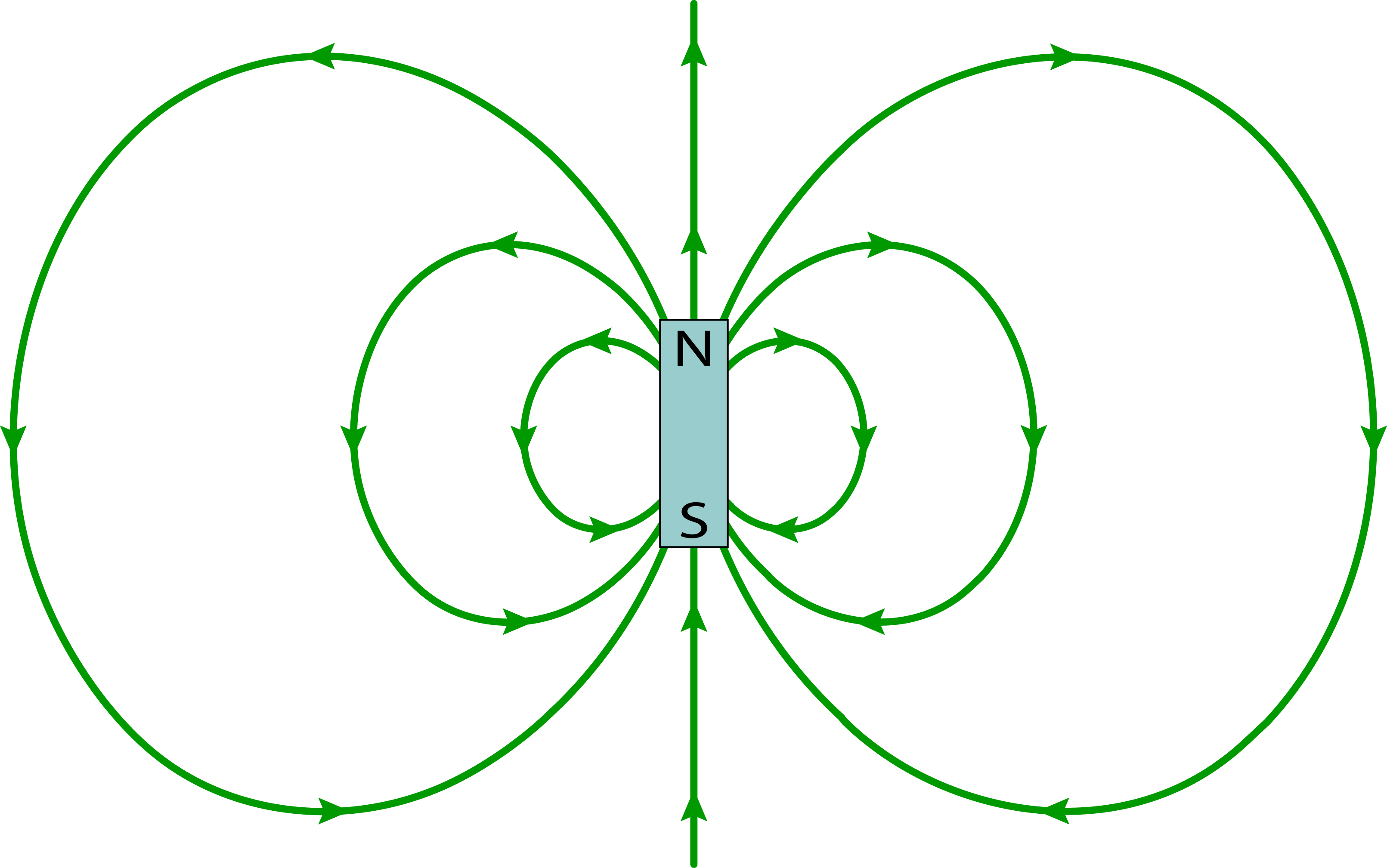
Fig. 1: A magnetic dipole field: magnetic field lines, shown in green, are generated by the two magnetic poles of a bar magnet.
The electric equivalent of this is shown in Fig. 2. If we just change the north and south magnetic poles into positive and negative electric charges, respectively, then the field generated becomes an electric field, and we get an electric dipole field, as you might expect.

Fig. 2: An electric dipole field. Electric field lines, shown in blue, as generated by two closely-spaced electric charges of magnitude ∣q∣ separated by a displacement vector $\vec d$.
What’s important here is the field itself, not the charges that generate it. In the case of subatomic particles like electrons, quarks, and neutrons, we can’t actually see the charges themselves - we can only measure the electric fields the particles generate. In principle, there’s no reason that these subatomic particles can’t produce the type of field shown in Fig. 2, even though we don’t think of any of them as two discrete, closely-spaced charges. Such a case is illustrated in Fig. 3. If any source of charge does create this type of field, we say that it possesses an electric dipole moment (edm), characterized by a vector $\vec p$. For example, a simple dipole like Fig. 2 has $\vec p = q\vec d$, where q is the magnitude of each charge (i.e., the positive monopole has charge q, while the negative one has charge − q) and $\vec d$ is the vector drawn from the negative charge to the positive charge, by convention. In the case of a single-particle dipole field like that of Fig. 3, the dipole vector $\vec p$ can be extracted from measurements of the field without ever making reference to q and $\vec d$ individually - which is good, because they don't even exist for this case. In other words, $\vec p$ is well-defined even in cases where q and $\vec d$ aren’t, which is why we say that it’s $\vec p$ that really matters.
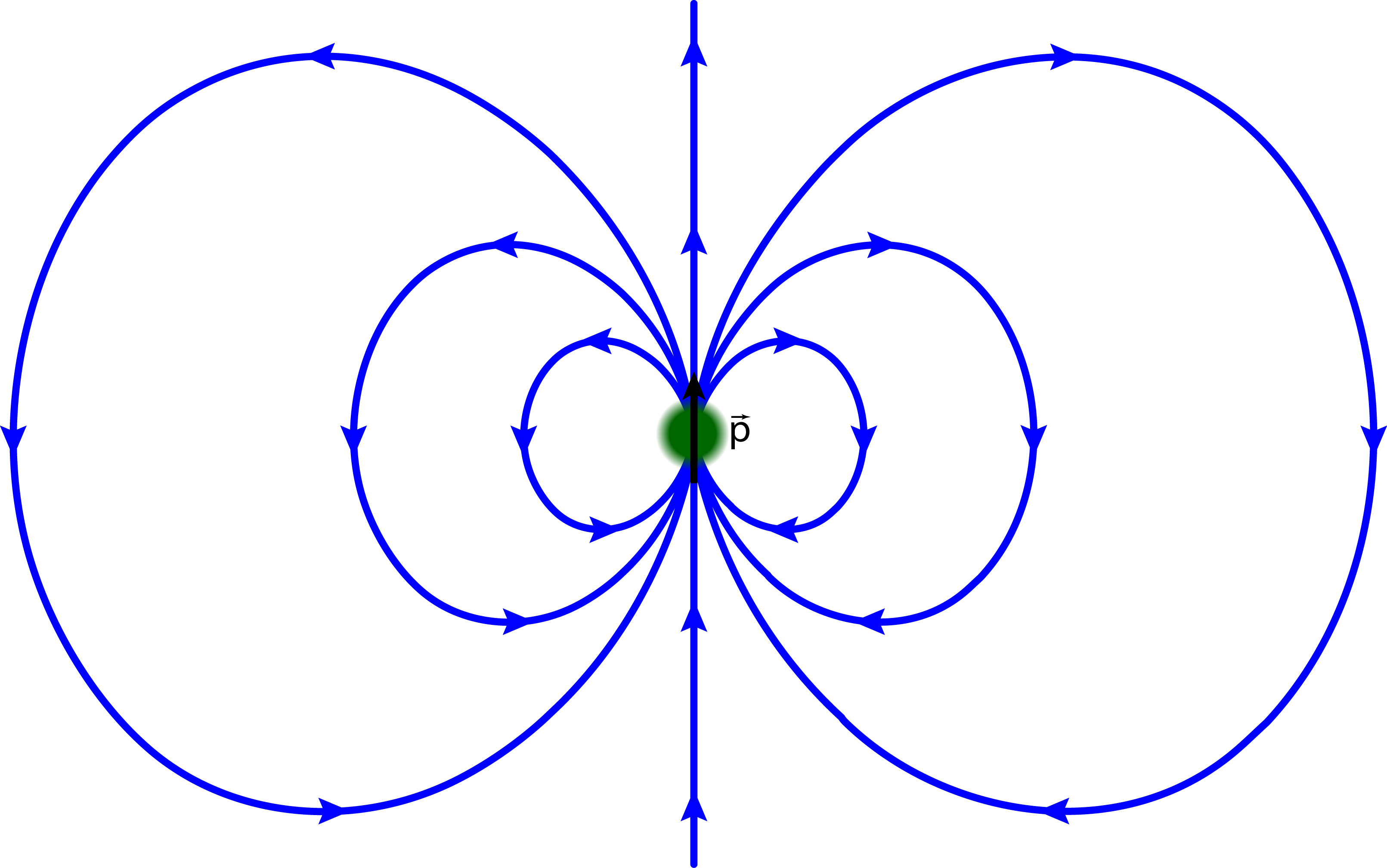
Fig. 3: An electric dipole field generated by a single particle. Even though we’ve never observed it, there’s no reason we know of that a particle can’t produce a dipole field even if it isn’t composed of two closely-spaced charges. The particle would then have an electric dipole moment $\vec p$. Note that the particle could be either electrically charged or electrically neutral; if charged, it would also generate an ordinary electric monopole field corresponding to its net charge.
It’s quite common for molecules to possess electric dipole moments (see Fig. 4 for the case of water, whose dipole moment is one of its highly important chemical properties), but these edms are not considered remarkable from the standpoint of physical theory. For pointlike particles like electrons and quarks to have edms, though, the violation of some fundamental symmetries is required, which makes them of great interest. The edms of fundamental particles are frequently called "permanent" edms to distinguish them from the edms of molecules, which are more frequently called simply "electric dipoles" or "dipole moments." If, say, an electron had a permanent edm, then the edms of all of the electrons in an atom would add up to give the atom as a whole its own edm. Even though the atom is composite instead of fundamental, its edm would still be a permanent edm. Similarly, the permanent edms of quarks would add together when three of them are bound into a neutron or proton, giving the larger particle its own permanent edm. Although molecular electric dipoles are commonplace, no permanent edm has ever been measured.
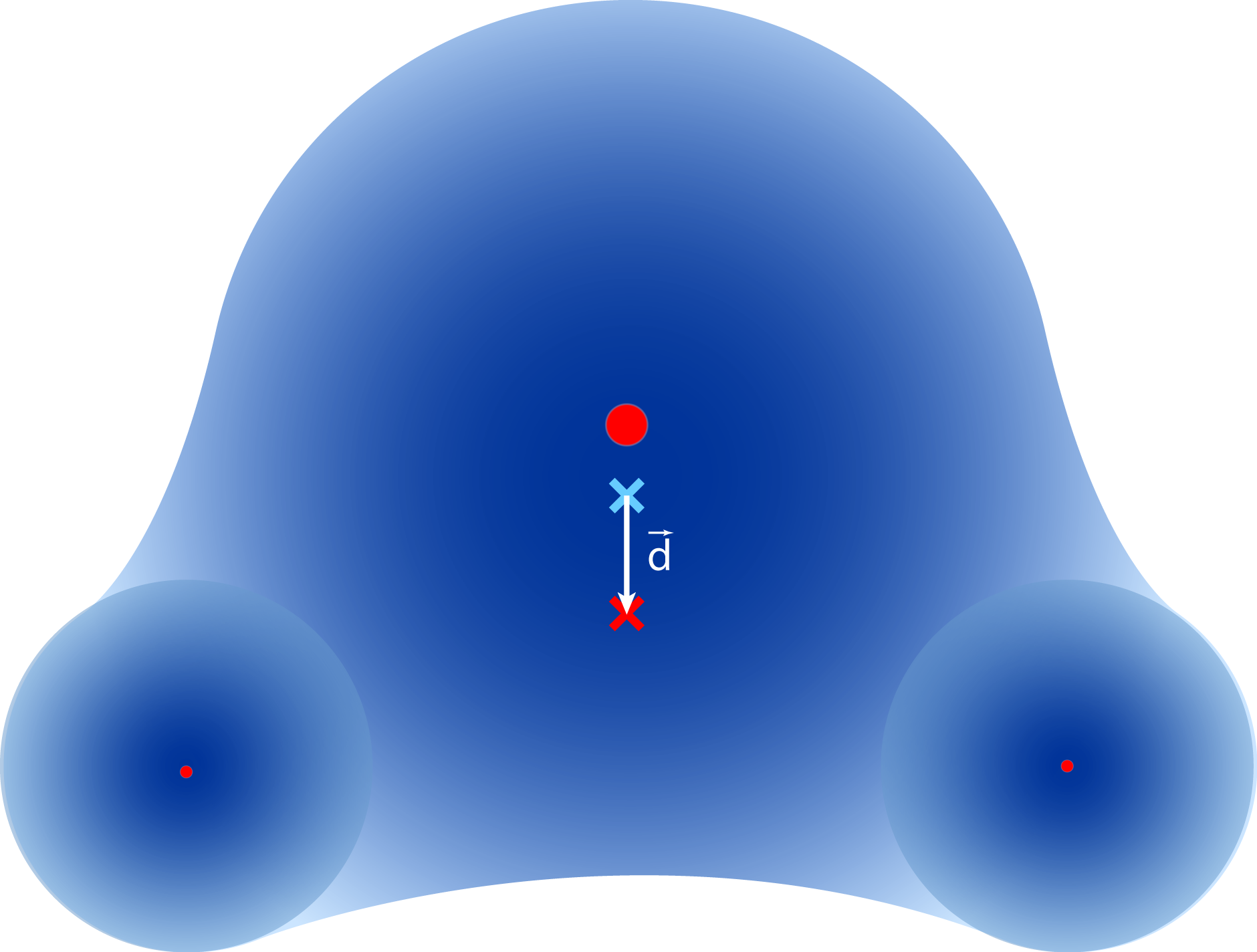
Fig. 4: A water molecule. The positive charge of the molecule is provided by the oxygen and two hydrogen nuclei, and the center of positive charge is represented by the red X. The negative charge is provided by the electron cloud, who are attracted to the highly-charged oxygen nucleus. This shifts their center of charge, marked by the blue X, slightly toward the oxygen nucleus, giving an overall net separation of charge to the molecule as indicated by the vector $\vec d$. This constitutes a dipole moment $\vec p $ of magnitude 1.85 Debye, or $3.85\times 10^{-9} e\,{\rm cm}$. The nuclei are magnified by a factor of about 1,000 for visibility; the magnitude of $\vec d$ is exaggerated by a factor of about 5.
Permanent edms
As alluded to above, the reason that we have special interest in permanent edms is that they allow the violation of time-reversal symmetry, which almost all laws of physics obey. More precisely, a particle with both a magnetic dipole moment and a permanent edm can be made to behave in two measurably different ways depending on whether time is flowing forward or backward! This may sound like Star Trek science-babble, but it’s a real concept and quite significant given that so few aspects of physical theory make this distinction with respect to the arrow of time. Of course, the "backwards time" case is only hypothetical, since we can’t actually reverse time to test it, but the fact that the symmetry violation shows up in the math is what’s noteworthy.
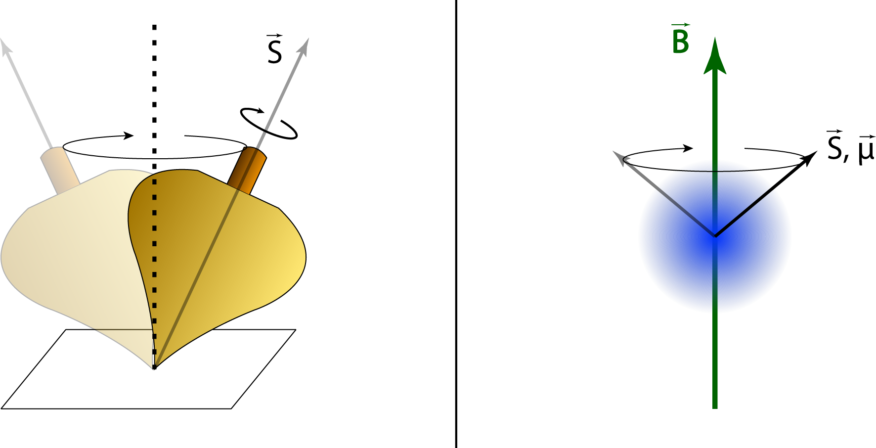
Fig. 5: Examples of precession. On the left, a top spins rapidly about its axis of symmetry (solid black line) while simultaneously precessing about a vertical line (dashed black line) at a slower rate. On the right, an electron displays the same behavior. The particle has a total angular momentum $\vec S$, called "spin," similar to that of a top spinning about its axis. Like the top, the particle precesses such that this vector traces out a cone around a magnetic field line $\vec B$.
This is how the time-reversal-symmetry violation would be realized. If you put a particle with an electric dipole moment in a uniform electric field, the particle will "wobble“ (the technical term is "precess") like a toy top about the external field lines, as shown in Fig. 5. The exact same thing happens to a particle with a magnetic dipole moment placed in a uniform magnetic field. In either case, you can measure the frequency of its precession - how many times per second the particle wobbles its way around the field line. If you put a particle with both electric and magnetic dipoles into uniform $\vec E$ and $\vec B$ fields, then it will have a net precession frequency that’s the sum of the two individual types. If you then take the equations that describe this precession and replace the time coordinate t with − t, mathematically "reversing" the flow of time, they give you a completely different number for the precession frequency! This is what it means when someone says that edms imply time-reversal asymmetry.
There’s a more concrete reason why permanent edm searches are important, though. The most fundamental theory of particle physics that we have is the Standard Model, which predicts that the electron and neutron do have nonzero edms (which itself is neat), but that they are so tiny that they are essentially immeasurable - millions or billions of times smaller than the smallest edm we’re capable of measuring today. Table 1 illustrates this for the cases of neutrons and electrons. The Standard Model predicts a neutron edm of $d_n \lesssim 10^{-32} \, e\,\text{cm}$, while the most precise experiment to date (reported in 2006) could measure only down to $d_n < 2.9 \times 10^{-26} \, e\, \rm{cm}$ ($e\, \rm{cm}$ is the typical unit used to measure permanent edms). That is, the predicted dn is 1,000,000 times smaller than the smallest dn we can possibly measure, as of May 2014. For the electron, the Standard Model predicts $d_e \lesssim 10^{-38} \, e\,\rm{cm}$, while the most precise experiment to date (reported in 2013) could measure only to $d_e < 8.7 \times 10^{-29} \, e\, \rm{cm}$ - nearly 10,000,000,000 times larger than the prediction! Clearly, the measurement of a Standard Model edm is not imminent, barring some sort of truly miraculous breakthrough in experimental technique. However, we know that the Standard Model is an incomplete description of the universe, and there are hundreds of theories proposing to extend or correct it - collectively, we refer to these as theories of "Physics Beyond the Standard Model." It turns out to be difficult to articulate such a theory that doesn’t give electrons and neutrons much larger edms - large enough, in fact, that they either should have been observed by now or will be soon. The fact that we haven’t seen a permanent edm allows us to place constraints on the free parameters of these theories, or even exclude them entirely. Searches for edms are therefore invaluable in figuring out where we should go from the Standard Model, now that the discovery of the Higgs Boson has nearly completed it.
| Particle | SM prediction | Observable limit |
|---|---|---|
| neutron | $10^{-32} \, e\,{\rm cm}$ | $< 2.9 \times 10^{-26} \, e\, {\rm cm}$ |
| electron | $10^{-38} \, e\,{\rm cm}$ | $< 8.7 \times 10^{-29} \, e\, \rm{cm}$ |
Physicists have been searching for permanent edms since the 1950’s, and many impressively precise experiments since have failed to measure anything. Observations have focused on measuring the edm of the neutron and the edms of certain atoms. Neither of these systems, you may notice, are fundamental particles. The atom consists of a nucleus (itself a wad of protons and neutrons) surrounded by a cloud of electrons, while the neutron is composed of three quarks (one up and two downs). Quarks and electrons are currently understood to be fundamental particles, and their edms, if they exist, would give edms to the neutron and to atoms, respectively. This is illustrated for the case of the neutron in Fig. 6.
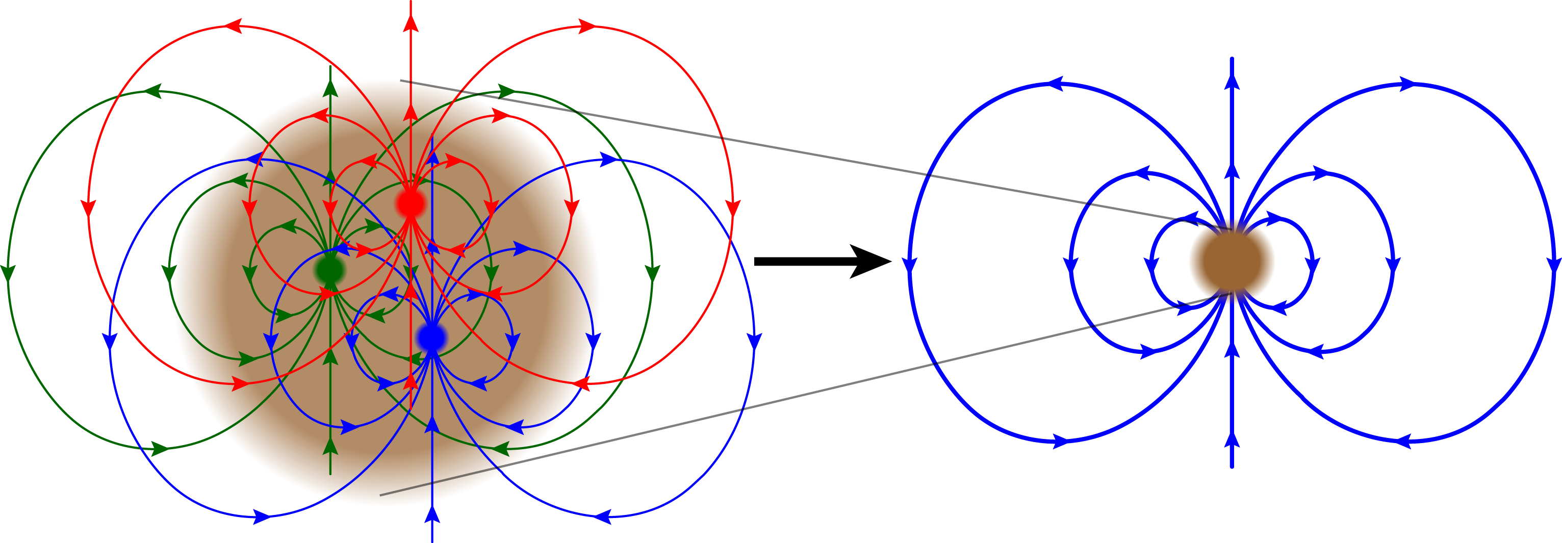
Fig. 6: A cartoon of the neutron (brown). The neutron contains three valence quarks: one red, one green, and one blue, shown on the left. If each quark has an edm, it will generate a dipole field like that of Fig. 3 (I’ve color-coded the fields generated by each quark individually for a modicum of clarity, but they're all electric dipole fields). Outside the neutron, shown on the right, the three fields will add together to produce an overall dipole field that, as far as an outside observer can tell, belongs to the neutron itself. Thus, the neutron gains a permanent edm due to those of its constituent quarks. In a similar way, electrons with edms will give an edm to the atom that they are a part of.
Research: edms in Composite Systems
This raises an important point, and one that takes us directly into the research at hand: if you’re looking for an electron edm by experimenting on atoms, what you’re really measuring is the edm of the atom. So, how is the edm of the atom $\vec d_{atom}$ related to the edm of its constituent electrons $\vec d_e$? Similarly, how does the neutron edm $\vec d_n$ depend on the edms of its quarks, $\vec d_u$ and $\vec d_d$? In order to interpret results from an experiment on atoms and neutrons in terms of the fundamental physics of electrons and quarks, it is vital to know these relationships. These two cases are the subject of this paper.
edms of Paramagnetic Atoms
In considering atoms, note first off that an atomic edm $\vec d_{atom}$ can be created both by its electrons having edms $\vec d_e$ and by its nucleus having an edm $\vec d_N$ (which would itself be due to proton and neutron edms). Nuclear edms might certainly exist, and many experiments are conducted to look for them. Primarily, these searches look at what are called "diamagnetic" atoms (mercury is a popular one), and they are researched by people other than me. In this paper, we focus only on the effects of electrons in producing an atomic edm.
So: how does $\vec d_{atom}$ depend on $\vec d_e$? At first glance, the answer seems quite simple when we consider how electrons pair up into orbitals in the atomic cloud. When this pairing happens, the total overall angular momentum and magnetic dipole moments of the two electrons align against each other to cancel out completely, and the same is true for the electric dipole moments as well. To measure any sort of atomic edm, then, we have to look in an atom with an unpaired electron, like that of sodium, illustrated in Fig. 7. Alkali atoms like sodium are perfect for exploring edms, since they are characterized by a single unpaired valence electron.
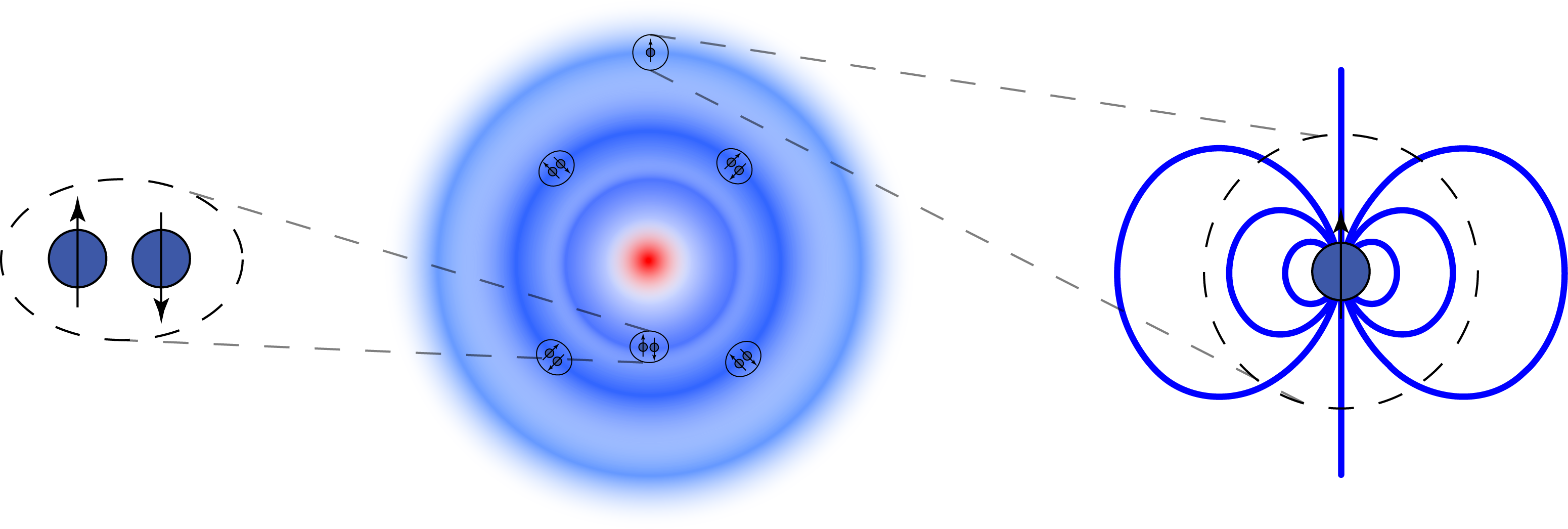
Fig. 7: A schematic of the sodium (Z=11) atom. The electrons of the two inner shells are paired into orbitals, as shown in the left inset. Any dipole moments the paired electrons might have cancel out, since they are anti-aligned with each other. The unpaired valence electron of the third shell, however, does not have its dipole field cancelled, and it therefore contributes to the dipole field of the entire atom.
Schiff's Theorem
So, the atomic edm is just the edm of this single electron: $\vec d_{atom} = \vec d_e$? At first order - neglecting all of the other electrons in the cloud, the ones paired up into orbitals - yes. We can’t really neglect all of the other electrons, though, because they’re all constantly exerting electromagnetic forces on the unpaired electron. When we consider these additional forces in the presence of the external electric field needed to probe the atom’s edm, it turns out that the electron cloud and the nucleus will reconfigure themselves in a way that always cancels out the lone electron’s edm. In other words, the only atomic edm we can ever measure is $\vec d_{atom} = 0$, even if $\vec d_e$ is nonzero! This result is known as Schiff’s Theorem.
Schiff’s Theorem seems like bad news, but fortunately there are two main loopholes that keep edm searches in atoms from being entirely futile. The first, familiar to nuclear physicists, is that the theorem assumes a point-like nucleus, which is untrue in practice. Again, we’re not concerned with the nucleus here, but you can research the "Schiff moment of the nucleus" if you’d like to learn more about how nuclear edms are investigated. The second loophole is that Schiff’s Theorem assumes nonrelativistic dynamics - that is, nothing in the atom is moving at an appreciable fraction of the speed of light. For hydrogen and light atoms, this is a perfectly good assumption. For heavy atoms, however, core electrons can be highly relativistic. As shown by Sandars, relativistic atoms do not necessarily reconfigure in the way Schiff predicted, and Schiff’s suppression of the edm can therefore be avoided. It gets better, though - not only is edm suppression avoided, but the atomic edm can even get bigger relative to the electron edm! That is, for $\vec d_{atom} = R\vec d_e$, where Schiff’s Theorem demands R = 0, Sandars showed that for relativistic atoms R can be on the order of 100 or even nearly 1000, depending on the atom - a remarkable result.
To understand why this is exciting, consider running an experiment whose equipment is intrinsically capable of measuring an edm as small as d = d0. If it were possible to measure an individual electron, it would need to have an edm at least as large as d0 to be seen. If the electron is in an atom with an enhancement factor of R = 100, though, it is the atom itself that must have an edm of at least d0. Assuming it does, and this $\vec d_{atom} = d_0$ is measured, then the enhancement factor implies that the original electron edm must have been $d_e = \frac1R\,d_0 = 0.01\,d_0$, 100 times smaller. Sandars enhancement in atoms therefore gives us the ability to measure electron edms much smaller than a given experimental apparatus would allow by itself.
A natural question is whether the same type of enhancement of electron edms when bound into an atom also happens with respect to quark edms when bound into a neutron. We’ll return to this question in the next section, but first we want to make sure the approach we have planned for the neutron works as expected when we apply it to the atom. If we can recreate Sandars’s results using our own technique, then we can be confident in its usefulness. This is the subject of the current section.
Before proceeding, we’ll need a short note for readers that don’t have physics backgrounds. The behavior of all of the atomic and subatomic particles we’ve discussed so far is governed by quantum theory, and quantum theory has two "tiers.“ The first can be called "ordinary quantum mechanics," that developed in the 1920’s. The Schrödinger and Dirac equations, which you may have heard of, are keystones of ordinary quantum mechanics. The second tier is "quantum field theory," developed in the 1950’s, which is more precise than ordinary quantum mechanics but also much more complicated mathematically. Quantum electrodynamics (QED), quantum chromodynamics (QCD), the Standard Model, and anything else involving Feynman diagrams are examples of quantum field theories. Ordinary quantum mechanics can be thought of as a low-energy approximation of a quantum field theory, and most physicists expect that the right quantum field theory (our current best guess is the Standard Model) will be an exact description of the fundamental laws of physics, though we’ll probably only be able to produce approximate solutions for it. Even though it’s not as exact, ordinary quantum mechanics is routinely used for calculations, since it’s much easier to work with than the more precise quantum field theory.
Sandars’s method for showing that relativistic atoms can evade Schiff’s theorem is based on ordinary quantum mechanics. It is mathematically sound, but the underlying physics responsible for it is not considered intuitive to most - I’ll admit that it certainly isn’t to me. The Sandars method starts with a complete description of the entire atomic system using ordinary quantum mechanics, accounting in principle for every electron and the nucleus individually and all of their interactions. It then distills from this description a specialized term that correctly describes the edm of the atom as a whole while making no explicit reference to the individual electrons or the way they interact.
In this paper, we use a completely different (and new!) approach to obtain the same results as Sandars for atomic edms. Our technique employs the quantum field theory of QED in a manner that is capable of fully and explicitly accounting for all of the electrons in the cloud and all of the ways they can interact with each other (in principle, at least). Naturally, it’s also much more involved and bulky, since this is a lot of stuff to account for. Our intent is not to replace the elegant Sandars calculation of atomic edms, only to show that it’s consistent with the quantum field theory approach we develop. The paper’s title begins with the phrase "Field theory calculation..." in order to emphasize this distinction between our method and that of Sandars.
The Furry representation
The key to accomplishing this field-theoretic calculation of edm enhancement in atoms is an idea from atomic physics called the Furry representation. The main idea of the Furry representation is that quantum field theory calculations can be made more efficient by first using ordinary quantum mechanics to guess the best starting approximations of the particles’ states. It’s called a "representation" because it uses these alternate solutions from ordinary quantum mechanics to represent the state of the particles when doing quantum field theory. Furry successfully applied this trick to the hydrogen atom, where the ordinary quantum mechanical states can be solved exactly; he used these simpler solutions as starting points for field-theoretical calculations of several important properties of the hydrogen atom.
In the present case, we can’t use Furry’s representation outright, because we’re not studying hydrogen. We’re studying multielectron atoms, and we can’t solve for the ordinary quantum mechanical states of a multielectron atom exactly. In such complicated, composite systems, any given electron feels not only the attractive force exerted by the nucleus, but also the repulsive forces exerted by every other electron in the atomic cloud. This tangle of interactions doesn’t just sound complicated, it’s a mathematical fact - Poincaré famously proved in the 19th century that systems of three or more interacting bodies like this cannot be solved exactly.
At the level of ordinary quantum mechanics, however, there are ways to approximate the effects of the rest of the electron cloud on any given electron by modeling the rest of the cloud as a sort of "screen" that keeps the individual electron from feeling the full attraction of the nucleus. This is done by introducing a screening potential when calculating the state of an electron using ordinary quantum mechanics. Screening potentials are generally well-grounded in physical reasoning, but at heart they are ad hoc constructions designed to model the states of electrons in the atomic cloud, not to predict them from first principles.
Our idea is to start with the Furry representation, but instead of exactly-known hydrogen states, we use screened electron states as the starting guess for field-theory calculations. It seems sort of obvious in some ways, but as far as we can tell, no one has done this before. We refer to it as a modified Furry Representation. In this research, we chose to use the Core Hartree screening potential after a co-author determined that it is most directly comparable to the Sandars method. Since we can’t determine the screened electron states exactly, we use a set of computer programs to calculate them to an excellent approximation.
The results are shown in Table 2, which is a simplified version of the ‘Table 1’ from the paper. In the paper, we break down the results in terms of specific Feynman diagrams, each representing a distinct physical process, which is more detail than warranted here. Z, the atomic number, is the number of protons in the nucleus of the atom, and thus correlates with how relativistic the atom’s core electrons are. The edm enhancement factor R is the key result of our calculations. We didn’t bother to include separate columns for our results and those of Sandars since, as expected, they’re exactly the same numbers. We can conclude that our two approaches are mathematically equivalent, even though they are quite different in execution.
| Atom | Z | R |
|---|---|---|
| Li | 3 | 0.004 |
| Na | 11 | 0.439 |
| K | 19 | 3.588 |
| Rb | 37 | 33.732 |
| Cs | 55 | 154.657 |
| Fr | 87 | 1066.891 |
| Tl | 81 | -792.665 |
Note that you can clearly see Schiff’s Theorem at work as the atoms get lighter and therefore more nonrelativistic - the "enhancement" factor for lithium is clearly more of a "dehancement" factor, reflecting nearly total Schiff suppression of the edm for this very nonrelativistic atom. Francium, on the other hand, displays an impressive three orders of magnitude enhancement of the edm! It would clearly make a powerful probe of the electron’s edm. Unfortunately, natural francium is so highly radioactive and its synthetic stable isotopes so difficult to produce that using it for this type of experiment is out of the question. Cesium, however, is lab-friendly and is used in edm searches such as the Electron EDM Project at LBNL.
You may have noticed that thallium, listed on the table, is not an alkali atom. Like the alkali elements, thallium has an unpaired electron, and it has a significant edm enhancement factor. Note that it has a minus sign; from $\vec d_{atom} = R\,\vec d_e$, this indicates that the overall edm vector of the atom is opposite in direction to the edm vector of the unpaired electron. Since we never see the edm vector of a lone electron, though, this sign doesn’t really matter. Alkali atoms and thallium are all examples of paramagnetic atoms, those that have magnetic dipole moments that can be aligned by external magnetic fields. The inclusion of thallium is why we refer to paramagnetic atoms, not just alkali atoms, in the title and text of the paper.
The edm of the Neutron
Our work in recreating the enhancement of certain atomic edms is interesting in its own right, but the original motivation for the research you’re reading about concerns the edm of the neutron. In particular, we wondered if the same long-established edm enhancement seen in some relativistic atoms due to electromagnetic interactions among the electrons might also appear in the neutron, since its quarks are also highly relativistic and electromagnetically interacting. The neutron is a bound state of one up quark and two down quarks, so in this case we want to find explicitly how the neutron edm dn depends on the quark edms du and dd. By analogy to the atomic case, we might write dn (du, dd) = Rudu + Rddd, where our task is to determine Ru and Rd.
At this point, you should try to set aside much of what you read just above about the atom. In particular, the interior of the neutron does not have its own atomic nucleus and does not have an electron cloud. There’s no Schiff’s Theorem and no screening, because these are behaviors of electron clouds. There is no Furry representation, modified or otherwise. There are only three quarks, whose behavior is determined by the nuclear strong force of quantum chromodynamics (QCD) but who also interact via the electromagnetic force of quantum electrodynamics (QED).
The relation between dn and du, dd has received plenty of attention before our research, of course, but it’s never been "solved," exactly. The fundamental problem with such calculations is that the states of the quarks within the neutron are determined primarily by QCD, with the weaker QED being a slight background (in atoms, there is no QCD force between the electrons and nucleus, so QED is dominant there). We know what the equations of QCD are, but they are much more difficult to solve than those of QED. When I say "much more difficult," I mean, "we don’t even really know how to with any precision yet." Instead, we have to rely on cruder approximation techniques, most of which are valid only for certain quark energies. Few of these are reliable for heavy bound states like the proton and neutron.
Nevertheless, we’ll review some estimates for how
dn depends on
du and
dd, just to get a feel for what
to expect. The most elementary way to estimate the relation we’re after is to ignore
both QCD and QED entirely and consider separate, noninteracting particles that just
happen to be near each other. This is sometimes called the SU(6) quark model. For
three such quarks, we can describe the possible states of each particle individually,
including their edms, and then use basic quantum mechanics to determine what overall
states are possible as combinations of the different individual states. I’ll skip the
math, but the edm of the overall state is found to be
$$d_n(d_u, d_d) = \frac43 d_d - \frac13 d_u.$$
This is
a pretty cartoonish zeroth-order approximation to the structure and edm of the neutron,
but it gives us a flavor of what type of answer we might end up with. In fact, we see
this same structure repeatedly when considering more precise estimates. One such example
is a more involved calculation using what are called the "QCD sum rules", and its
result is
$$\label{eq:SumRules = Eq. 1}
d_n = (1 \pm 0.5)\frac{| \langle \bar{q}q \rangle |}{(225 \rm{MeV})^3}
\left[ 1.1e(\tilde{d}_d + 0.5\tilde{d}_u) + 1.4(d_d - 0.25 d_u)\right].$$
This expression probably appears pretty arcane to you, and to be honest it’s not much better for me. Nevertheless, it’s a worthwhile exercise to examine it more closely, just to see what we can learn from it. If you don’t care to, you can skip the next paragraph without losing too much of the train of thought of the paper, since this result doesn’t affect the research results presented later. Note that what I’m about to discuss is outside my area of expertise, so A) don’t take anything in it as a fact and B) if this is your area of expertise, please feel free to email me (caretaker@TheScienceMill.com) with corrections or elaborations. I’d love to learn more about this.
First of all, the factor (1 ± 0.5) tells us right away that the rest of the expression can only be considered accurate to within about 50%. Anything involving QCD is, unfortunately, going to be fundamentally imprecise like this. The factor ∣⟨q̄q⟩∣ represents the quark condensate, which is essentially a measure of the "quarkness density“ of the vacuum, a way of approximating the effects of unobservable quark-antiquark pairs that pop in and out of the vacuum continually. It can’t be calculated precisely, and as far as I know it can only vaguely be extracted from experimental data, which is why it’s left in symbolic form. I presume, though, that its value is expected to be something along the lines of $(225 \rm{MeV})^3$, since that’s about the only reason I can imagine that this particular number would be extracted explicitly. Overall, then, the entire factor of $\frac{| \langle \bar{q}q \rangle |}{(225 \rm{MeV})^3} \approx 1$. The real action is within the square brackets. The quantities d̃d and d̃u are the chromoelectric dipole moments of the down and up quarks. If the electric dipole moment measures the overall separation of electric charge as in Fig. 2, then the chromoelectric dipole moment measures the overall separation of color charge, the type of charge that quarks possess that makes them responsive to the strong force. Color charge is entirely separate from electric charge, yet color charge dipoles show up explicitly in modeling the electric charge dipole of the neutron! Since I have no tools for working with chromo-edms, and they’re irrelevant to the research I’m explaining, I’ll have to neglect this intriguing development for the remainder of the discussion. We’re now left with the quantity 1.4(dd − 0.25du), which you’ll notice is numerically quite similar to the $\frac43 d_d - \frac13 d_u$ that I said would keep cropping up. After all the work we’ve done to interpret Eq. 1, what we end up with is: "Except for the influence of chromo-edms, it’s basically the same as the simplistic SU(6) result."
These and other methods for estimating dn (du, dd) come to the same broad conclusion that the neutron edm is about the same size as the quark edms - there’s neither suppression (like we saw with Schiff’s theorem) nor enhancement (like we saw with the relativistic atoms of Sandars). What our approach offers toward estimating dn(du, dd) that these other methods do not is that we explicitly evaluate corrections to the neutron’s structure generated by electromagnetic interactions among the quarks. These corrections are where the edm enhancement occurs in heavy atoms, so we should expect that if the same phenomenon exists in the neutron, then only a method such as ours would reveal it.
Our solution for dealing with the intransigence of QCD is to recognize that, fundamentally, we’re not calculating a QCD effect. Instead, we’re estimating an electromagnetic effect in a system whose state happens to be determined primarily by QCD. This is the type of problem the cavity model is appropriate for addressing. The cavity model deserves (and will soon receive) its own exposition, but for now what’s important to know is that it gives us approximations for the states of the quarks, which serve a similar function to the screened electron states we used when doing atoms above. The cavity quark states are less precise approximations than the screened electron states, but they should still suffice for our purposes. Once we have these quark states, we can begin to calculate what effect their interactions have on the overall edm of the neutron.
Results
Our field theoretic approach is what we call perturbative, meaning that we don’t
calculate the entire answer all at once. Instead, we break it into chunks and calculate only
the most important chunks, with "importance" determined by how much of the answer we expect
that chunk to contain. At first order (the most important chunk), we end up with
$$d_n^{(1)}(d_u, d_d) = (0.8265)\left( \frac43 d_d - \frac13 d_u \right)$$
in the cavity model, which is noticeably similar to the SU(6) result. This isn’t surprising,
since the cavity model at first order completely neglects any interactions among the quarks,
so it’s essentially just the SU(6) case squeezed into a hard sphere. Accounting for this binding
effect results in a 17% reduction in dn that
the SU(6) estimate ignores. This is also perfectly compatible with the more complicated Eq. 1
and its (rather wide) error bars.
Second order brings in the electromagnetic interactions among the quarks, and this is where we would
expect the edm enhancement to show up if it exists. Our result is
$$d_n^{(2)}(d_u, d_d) = 2.51 × 10^{−4} d_u - 1.60 × 10^{-3} d_d $$
Notice that these are very small numbers! Compared
to the first order result, these are negligible, and they certainly cannot be interpreted as enhancements.
We conclude that the enhancement of the electron’s edm in certain heavy atoms due to electromagnetic
corrections does not exist for the edms of quarks in a neutron.
Why aren’t there edm enhancements in the neutron? Mathematically, in the process of deriving our results, we notice that the equations that give d n(2) all contain a factor of $\frac{1}{E_n - E_0}$, where E0 is the quarks’ lowest-energy state inside the neutron, where they spend most of their time, and En is some higher-energy state that the quark can gain from interactions with the other quarks. This factor is typical of second-order perturbation theory. These energy states are determined by the QCD equations, and thus the quantity En − E0 characterizes the energy scale of QCD interactions. It’s typically $\sim 100\,{\rm MeV}$. By contrast, the corresponding factor in the atomic case is $\sim 10\,{\rm eV}$, which value characterizes the energy scale of the electromagnetic interactions that govern the atom. In moving from the atom to the neutron - that is, moving from an environment dominated by the relatively weak QED to one dominated by the stronger QCD - this factor translates as $\frac{1}{10\,{\rm eV}} \rightarrow \frac{1}{100\,{\rm MeV}}$, a reduction of 10 − 7. If we assume that the relativistic electromagnetic force does tend to produce edm enhancement factor of, say, R = 103, comparable to that of thallium or francium, then including the force-conversion reduction factor of 10 − 7 brings this down to the level of 10 − 4 overall, which is exactly what we see. Physically, the idea is this: the electromagnetic forces responsible for edm enhancement are far too weak to affect the structure of a bound state held together by the powerful influence of QCD. It is called the "strong force" for a reason, after all.
This is the end result of the paper, but it leaves open an intriguing window that I’d love to pursue if I ever get the chance. With reference to Eq. 1, recall that the edm of the neutron is affected by the chromo-edms of the quarks. Even though the electromagnetic force is suppressed in a QCD environment, the possibility remains that relativistic QCD interactions among the chromo-edms can enhance the dependence of dn on d̃u and d̃d in the same way that electromagnetic interactions enhance edms in the atomic environment. Essentially, by examining the force most relevant to the environment, the same underlying physics may still be at work. Unfortunately, none of the tools we’ve developed to work with ordinary edms would apply usefully to problems of chromo-edms, so we’d have to go all the way back to the drawing board!